
The Finite Element Method (FEM) is a powerful numerical technique widely used in engineering, physics, and various scientific disciplines to solve complex problems with practical applications. This article aims to provide a comprehensive understanding of the Finite Element Method, discussing its theoretical foundations, the discretization process, implementation, and real-world applications. By delving into the intricacies of FEM, readers will gain insight into its strengths, limitations, and potential for solving diverse engineering challenges.
What Is The Finite Element Method (FEM)
The Finite Element Method (FEM) is a numerical technique used to solve a wide range of complex engineering, physics, and scientific problems. It provides a systematic approach for approximating and solving differential equations that describe various physical phenomena, such as heat transfer, structural analysis, fluid dynamics, electromagnetics, and many others.
FEM is particularly well-suited for problems with irregular geometries, complex boundary conditions, and varying material properties.
At its core, the Finite Element Method involves dividing a continuous domain into smaller, simpler sub-domains called “finite elements.” These elements are geometric shapes (e.g., triangles, quadrilaterals, tetrahedra, or hexahedra) that collectively approximate the original domain. The process of dividing the domain into finite elements is known as discretization.By discretizing the domain, FEM transforms the problem into a set of algebraic equations, making it amenable to computer-based numerical analysis.
1.Steps Of Finite Element Method
The main steps involved in the Finite Element Method are as follows:
- Discretization: The continuous domain is divided into smaller finite elements. The choice of element type and size depends on the problem’s nature and complexity.
- Approximation: Within each finite element, approximate functions, known as “shape functions” or “interpolation functions,” are used to describe the behavior of the unknowns (e.g., displacements, temperature, pressure, etc.). These shape functions are usually simple polynomials and enable the representation of the solution across the entire domain.
- Weak Formulation: The governing differential equations describing the physical behavior (e.g., partial differential equations) are converted into integral equations through the application of variational principles. This process is called weak formulation or the principle of minimum potential energy.
- Assembly: The elemental equations from each finite element are combined to form a global system of equations that represents the entire problem. This process involves the assembly of stiffness matrices and load vectors, accounting for the interactions and continuity between neighboring elements.
- Boundary Conditions: Essential boundary conditions (e.g., fixed displacements, temperature, etc.) and natural boundary conditions (e.g., external forces, heat fluxes) are imposed on the global system to model the real-world constraints and interactions.
- Solution: The resulting system of equations is solved numerically using various methods, such as direct solvers or iterative techniques. The unknown values of the problem (e.g., displacements, temperature distribution) are obtained through this process.
- Post-processing: After obtaining the numerical solution, post-processing is performed to extract the desired quantities of interest and visualize the results.
The Finite Element Method offers several advantages, including its ability to handle complex geometries, variable material properties, and boundary conditions. Additionally, FEM allows for easy refinement of the mesh in regions of interest, providing higher accuracy where needed while reducing computational costs in less critical areas.
FEM has become an indispensable tool in engineering design, analysis, and optimization, enabling engineers and scientists to simulate and predict the behavior of complex systems without the need for costly and time-consuming physical prototyping. As computational capabilities continue to advance, the Finite Element Method continues to find applications in a wide range of industries and scientific fields.
Overview Of Numerical Methods In Engineering
Numerical methods, including the Finite Element Method (FEM), play a vital role in engineering by providing efficient and accurate solutions to complex problems that are challenging or impossible to solve analytically. These methods involve the use of mathematical algorithms and computational techniques to approximate and solve differential equations or other mathematical models that describe various physical phenomena encountered in engineering applications. Here’s an overview of some commonly used numerical methods in engineering, with a focus on the Finite Element Method:
Finite Difference Method (FDM)
The Finite Difference Method approximates derivatives in differential equations using discrete difference quotients. It is particularly useful for solving partial differential equations (PDEs) in one or more spatial dimensions and is widely used for problems involving heat transfer, fluid dynamics, and structural analysis. The method discretizes the domain into a grid, and the unknowns are represented at discrete points. FDM is relatively straightforward to implement but may be limited in handling irregular geometries.
Finite Volume Method (FVM)
The Finite Volume Method is commonly used to solve conservation laws in physics and engineering, such as fluid flow and heat transfer problems. It divides the domain into control volumes and computes the average values of the variables within each volume. The method balances the fluxes across the control volume boundaries and ensures that the conservation laws are satisfied. FVM is well-suited for problems with complex geometries and unstructured grids.
Finite Element Method (FEM)
As discussed earlier, the Finite Element Method is a versatile numerical technique widely used in engineering. It discretizes the domain into smaller finite elements, approximates the unknowns using shape functions, and formulates the problem as a system of algebraic equations. FEM is known for its ability to handle irregular geometries, varying material properties, and complex boundary conditions. It is widely used in structural analysis, heat transfer, fluid dynamics, and electromagnetic simulations, among other applications.
Boundary Element Method (BEM)
The Boundary Element Method focuses on discretizing only the boundary of the domain rather than the entire volume. It is particularly useful for problems involving Laplace’s equation, Poisson’s equation, and other elliptic PDEs. BEM offers advantages in problems with unbounded domains and reduces the computational effort by converting the problem’s dimensionality. It is often used for problems related to potential flows, electrostatics, and stress analysis.
Finite Analytical Method (FAM)
The Finite Analytical Method combines analytical and numerical approaches to solve differential equations. It uses analytical solutions for simple regions and employs numerical techniques like FEM or FDM for more complex regions. FAM aims to retain the accuracy of analytical methods while extending their application to complex geometries.
Meshless Methods
Meshless methods, including the Element-Free Galerkin (EFG) method and the Smoothed Particle Hydrodynamics (SPH) method, do not require a fixed mesh like FEM or FVM. Instead, they rely on scattered data points or particles to represent the domain. Meshless methods are advantageous in problems with extreme deformations, moving boundaries, and adaptive mesh requirements.
Each numerical method has its strengths and limitations, and the choice of method depends on the specific problem’s characteristics and the required computational resources. Engineers often employ a combination of these methods to tackle diverse engineering challenges, gaining valuable insights and predictions that facilitate the design and analysis of complex systems.
Theoretical Foundations of Finite Element Method
The Finite Element Method (FEM) is founded on mathematical principles derived from continuum mechanics and variational calculus. Understanding these theoretical foundations is essential for grasping the fundamental principles that underpin the FEM’s computational approach. Here are the key theoretical foundations of the Finite Element Method:
- Partial Differential Equations (PDEs) and Continuum Mechanics: At the heart of the FEM lies the governing partial differential equations that describe the physical behavior of the problem under consideration. These PDEs express the relationships between the unknowns (e.g., displacement, temperature, pressure) and their spatial and temporal variations. In engineering, these equations arise from the principles of conservation of mass, momentum, energy, and other fundamental laws governing the behavior of continua (solid, fluid, or heat-conducting materials).
- Variational Formulation: The Finite Element Method employs variational principles to formulate the problem in a weak form. The weak form is an integral formulation of the PDEs that leads to a set of integral equations. This approach, also known as the principle of minimum potential energy, simplifies the process of deriving the weak form of the problem. In the weak form, the differential equations are multiplied by test functions, and the resulting equations are integrated over the domain. The test functions serve as weighting functions, and the integral equations are expressed in terms of unknowns and their derivatives.
- Principle of Minimum Potential Energy: The principle of minimum potential energy is a variational principle that serves as the theoretical basis for the weak form of the PDEs. It states that a system in equilibrium achieves a configuration with the minimum potential energy. By expressing the problem in the weak form, the FEM transforms the differential equations into integral equations, allowing for easier manipulation and approximation.
- Galerkin Method: The Galerkin method is a specific type of weighted residual method employed in the FEM. It involves using the same set of functions (shape functions) for both the approximation of the unknowns and the test functions in the weak form. The Galerkin method ensures that the approximation errors and residual errors are orthogonal, leading to more accurate solutions.
- Shape Functions and Interpolation: The discretization process in the Finite Element Method involves approximating the unknowns within each finite element using shape functions. These shape functions are interpolation functions that describe the behavior of the unknowns within each element. They are chosen to be polynomials with specific properties to satisfy continuity requirements and to represent the approximate solution efficiently.
- Element Stiffness Matrix and Load Vector: The Finite Element Method discretizes the domain into smaller finite elements, and each element contributes to the global system of equations. The element stiffness matrix and load vector are derived using the weak form and the shape functions. The stiffness matrix relates the nodal displacements of an element to the internal forces and moments within that element. The load vector accounts for the external forces acting on the element.
- Global Assembly: Once the element stiffness matrices and load vectors are computed, they are assembled into the global stiffness matrix and load vector. Global assembly involves combining the contributions from all elements to form the complete system of equations for the entire problem domain.
By understanding these theoretical foundations, engineers and researchers can better appreciate the mathematical underpinnings of the Finite Element Method and its ability to solve complex engineering problems with accuracy and efficiency. These principles also lay the groundwork for further advancements and extensions of the FEM in handling more challenging and multi-physics problems.
Mesh Generation
Mesh generation is a crucial step in the Finite Element Method (FEM) where the continuous domain is discretized into smaller finite elements. These elements serve as building blocks for approximating the solution to the governing partial differential equations (PDEs) over the entire domain. The mesh should be structured or unstructured, depending on the complexity of the geometry and the required accuracy.
The primary element types used in FEM are 1D, 2D, and 3D elements.
- 1D Elements: 1D elements are used for problems with one spatial dimension, such as beam bending or heat conduction along a line. The most common 1D element is the “beam” or “rod” element, represented by two nodes connected by a line. The unknown variable (e.g., displacement, temperature) is typically interpolated linearly between these two nodes.
- 2D Elements: 2D elements are employed for problems involving two spatial dimensions, such as plane stress, plane strain, and heat conduction in a plate. The commonly used 2D elements include triangles (e.g., linear and quadratic triangles) and quadrilaterals (e.g., bilinear and biquadratic quadrilaterals). The nodes of these elements define their shape and size.
- 3D Elements: 3D elements are suitable for problems in three spatial dimensions, such as solid mechanics, fluid flow in a volume, and heat conduction in a solid. Commonly used 3D elements include tetrahedra (e.g., linear and quadratic tetrahedra) and hexahedra (e.g., bilinear and biquadratic hexahedra). These elements provide flexibility in accurately representing complex 3D geometries.
Shape Functions and Interpolation
Shape functions are mathematical functions used to interpolate the values of the unknown variables (e.g., displacement, temperature) within each finite element. These functions describe how the values vary within the element based on the values at the element’s nodes. Shape functions play a significant role in the approximation process and the assembly of element matrices and vectors.
For each type of element (e.g., linear triangle, bilinear quadrilateral), specific shape functions are used to approximate the unknown variables. These shape functions are chosen to satisfy essential properties, such as continuity between adjacent elements and the ability to represent different polynomial orders for higher accuracy.
Element Stiffness Matrix and Load Vector Assembly
The stiffness matrix and load vector for each finite element are derived based on the element’s shape functions, material properties, and geometry. The stiffness matrix represents the relationship between the nodal displacements and the internal forces and moments within the element. It is symmetric and positive definite for linear elastic materials.
The load vector contains the contributions of external forces or heat loads applied to the element. The assembly of the stiffness matrix and load vector involves numerical integration over the element’s domain using numerical quadrature techniques.
Global Assembly and Imposition of Boundary Conditions
Once the element stiffness matrices and load vectors are computed, they are assembled into the global stiffness matrix and load vector for the entire problem domain. Global assembly involves combining the contributions from all elements by mapping the element degrees of freedom to the global degrees of freedom.
Boundary conditions are essential constraints that mimic the real-world constraints and interactions. Essential boundary conditions, such as fixed displacements or prescribed temperatures, are imposed directly on the global system. Natural boundary conditions, such as external forces or heat fluxes, are incorporated through the load vector. The imposition of boundary conditions results in a reduced system of equations, leading to the final solution for the unknown variables.
Mesh generation, shape functions, element stiffness matrix and load vector assembly, global assembly, and imposition of boundary conditions are foundational steps in the Finite Element Method, enabling engineers to approximate and solve complex engineering problems with high accuracy and efficiency.
Applications of Finite Element Method
The Finite Element Method (FEM) is an incredibly versatile numerical technique with a wide range of applications across various engineering and scientific disciplines. Some of the key applications of FEM include:
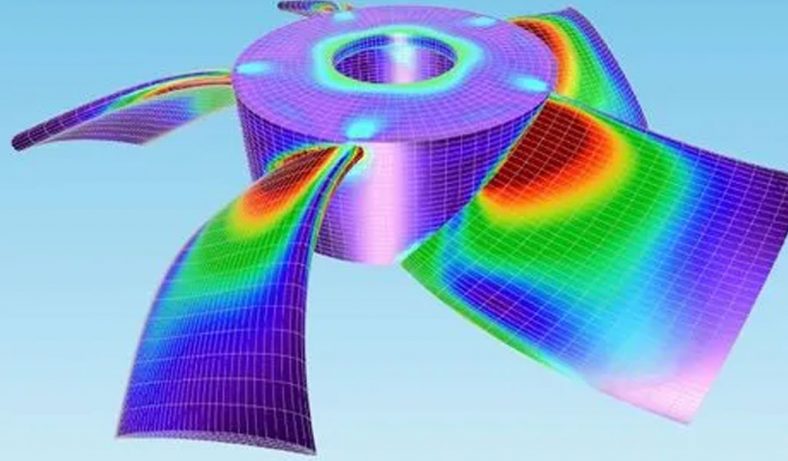
Structural Analysis
FEM is extensively used in structural engineering to analyze the behavior of structures under various loads and boundary conditions. It enables engineers to assess stress distributions, deformations, and stability of structures like bridges, buildings, aircraft, and mechanical components. Structural analysis helps ensure that designs meet safety requirements and can withstand real-world operating conditions.
Heat Transfer Analysis and Thermal Problems
FEM is employed to model heat conduction, convection, and radiation in solid structures and fluid domains. It finds applications in designing and analyzing heat exchangers, electronics cooling systems, thermal shields, and other heat transfer devices. FEM enables the prediction of temperature distributions and heat fluxes, facilitating optimal thermal management in engineering designs.
Fluid Dynamics and Computational Fluid Dynamics (CFD)
CFD simulations based on FEM are used to study fluid flow patterns, pressure distributions, and other fluid-related phenomena in complex geometries. This application is essential in designing efficient aerodynamics for aircraft and automobiles, optimizing industrial processes involving fluid flow, and predicting weather patterns and environmental impacts.
Electromagnetic Field Simulations
FEM is employed to analyze electromagnetic fields and interactions in a variety of devices and systems. It finds applications in designing antennas, electromagnetic sensors, transformers, motors, and electromagnetic compatibility (EMC) studies. Electromagnetic simulations are crucial for ensuring optimal performance and minimizing interference in electronic devices.
Acoustic and Vibration Analysis
FEM-based acoustic simulations are used to study sound propagation, noise radiation, and acoustic resonances in structures. This application is vital for designing quieter products, predicting noise levels in urban areas, and optimizing noise control measures. In addition, FEM is used to analyze the vibration behavior of structures and mechanical systems, aiding in identifying resonant frequencies and designing vibration isolation systems.
Multi-physics Simulations and Coupled Problems
FEM excels at handling multi-physics problems that involve the interaction of multiple physical phenomena. Examples include fluid-structure interaction (FSI), where fluid flow affects structural behavior, and thermo-mechanical coupling, where temperature changes induce mechanical deformations. FEM’s ability to handle coupled problems enables engineers to study complex systems where different physical processes influence each other.
The applications listed above represent just a fraction of the diverse areas where FEM is utilized. In practice, FEM is continually expanding its reach, playing an indispensable role in research, design, and optimization across numerous fields, including geomechanics, geophysics, medical imaging, material science, and more. As computational power increases and FEM techniques advance, its potential for solving complex problems continues to grow, driving innovation and progress in various industries.
Advancements and Extensions
Advancements and extensions in the Finite Element Method (FEM) have led to significant improvements in its efficiency, accuracy, and applicability to a broader range of problems. Here are some key advancements and extensions:
- Adaptive Mesh Refinement and Error Estimation: Adaptive mesh refinement (AMR) is a technique that dynamically adjusts the mesh resolution based on the solution’s error. Areas with high gradients or significant changes in the solution receive a finer mesh, while regions with low variation use coarser elements. AMR helps concentrate computational effort where it is most needed, leading to more accurate results while reducing computational resources. Error estimation techniques, such as the Zienkiewicz-Zhu error estimator, guide the mesh refinement process by quantifying the local error in the solution.
- Isogeometric Analysis and Higher-Order Elements: Isogeometric Analysis (IGA) is an integration of CAD (Computer-Aided Design) and FEM, where the same basis functions used for representing the geometry in CAD are utilized for the FEM solution. IGA facilitates smoother and more accurate solutions due to the use of high-degree B-spline or NURBS (Non-Uniform Rational B-Splines) basis functions, enabling higher-order continuity. This approach allows for seamless shape optimization, easier geometry modification, and reduced geometry-to-analysis meshing efforts.
- Meshless Methods and Their Advantages: Meshless methods, also known as mesh-free methods, eliminate the need for structured meshes. Instead, they use scattered data points or particles to represent the domain. Examples of meshless methods include the Element-Free Galerkin (EFG) method and the Smoothed Particle Hydrodynamics (SPH) method. Meshless methods are advantageous for problems involving moving boundaries, large deformations, and complex geometries. They offer better adaptability and simpler handling of domain changes compared to traditional mesh-based FEM.
- Hybrid FEM and Other Numerical Techniques: Hybrid FEM combines different numerical techniques within a single simulation to exploit the strengths of each method. For instance, it can employ FEM for the solid region and FVM (Finite Volume Method) for the fluid region in a fluid-structure interaction problem. Hybrid FEM allows for more accurate representation of the physics and smoother coupling between different domains. Besides hybridization, various other numerical techniques, such as extended FEM, generalized FEM, and smoothed FEM, have emerged to address specific challenges or improve efficiency in certain applications.
- FEM in Non-linear Analysis and Material Modeling: Non-linear analysis extends FEM to handle problems involving large deformations, material non-linearity, contact interactions, and other complex behaviors. Non-linear finite element simulations are crucial in applications like elastoplasticity, hyperelasticity, and creep analysis. Material modeling advancements, including incorporating more realistic material properties and damage models, allow FEM to simulate materials with varying behaviors under different loading conditions more accurately.
These advancements and extensions have expanded the capabilities of FEM and its applicability to a wider range of problems in engineering and scientific research. By integrating sophisticated techniques, handling non-linearities, and adapting the mesh to the problem’s demands, FEM continues to be a powerful tool for solving complex and realistic problems in various fields. As computational resources grow, further advancements and innovations in FEM are expected, enabling even more comprehensive simulations and analyses of intricate systems.