
Bernoulli’s equation is a fundamental principle in fluid dynamics, governing the behavior of fluid flow in various real-world scenarios. Developed by Swiss mathematician Daniel Bernoulli in the 18th century, the equation describes the relationship between pressure, velocity, and elevation in a moving fluid.
This comprehensive article delves into the historical context of Bernoulli’s discovery, the derivation and components of the equation, its applications in diverse fields, and the limitations and extensions in modern fluid dynamics. We explore practical examples and theoretical insights, unraveling the intricacies of this crucial equation and its enduring impact on engineering, aviation, hydraulics, and more.
The Define Of Bernoulli’s Equation
Bernoulli’s equation is a fundamental principle in fluid dynamics that describes the behavior of an incompressible and inviscid fluid as it flows through a closed system. It establishes a relationship between the pressure, velocity, and elevation of the fluid at different points along its path. Named after Swiss mathematician Daniel Bernoulli, who formulated it in the 18th century, the equation is based on the principle of conservation of energy applied to fluid flow.
In its simplest form, Bernoulli’s equation can be expressed as:P+21ρv2+ρgh=constant
P + \frac{1}{2}\rho v^2 + \rho gh = \text{constant}P+21ρv2+ρgh=constant
Where: PP = Pressure of the fluid
\rhoρ = Density of the fluid
vv = Velocity of the fluid
gg = Acceleration due to gravity
hh = Elevation or height of the fluid
Explanation of Terms:
- Pressure (PP): Pressure refers to the force exerted by the fluid on the walls of the container or conduit that contains it. In Bernoulli’s equation, it represents the static pressure of the fluid, which is the pressure due to the random motion of fluid molecules. As the fluid flows through a conduit, variations in the conduit’s cross-sectional area can cause changes in the fluid’s pressure.
- Kinetic Energy (\frac{1}{2}\rho v^221ρv2): The second term in the equation represents the kinetic energy of the fluid, where \rhoρ is the density of the fluid and vv is the velocity of the fluid. This term accounts for the energy associated with the fluid’s motion. When the fluid speeds up, its kinetic energy increases, and when it slows down, its kinetic energy decreases.
- Potential Energy (\rho ghρgh): The third term in the equation represents the potential energy of the fluid, where \rhoρ is the density of the fluid, gg is the acceleration due to gravity, and hh is the elevation or height of the fluid above a reference level. This term accounts for the energy associated with the fluid’s position in a gravitational field. An increase in elevation leads to an increase in potential energy, and a decrease in elevation leads to a decrease in potential energy.
- Constant: The sum of pressure, kinetic energy, and potential energy in the equation remains constant for a given fluid flow along a streamline in an idealized situation. This constant value is often referred to as the “total energy” or “Bernoulli’s constant” for the fluid flow.
Assumptions and Limitations:
It’s important to note that Bernoulli’s equation is based on certain assumptions and has limitations. The equation assumes that the fluid is incompressible (i.e., its density remains constant), inviscid (i.e., no internal friction or viscosity), and flows in a steady state along a streamline. Additionally, it assumes that the fluid flow is free of turbulence, and there are no external forces acting on the fluid (except gravity).
Real-World Applications:
Despite its idealized assumptions, Bernoulli’s equation finds extensive applications in various fields, including:
- Aviation: Bernoulli’s equation explains the principles of lift generation that allow airplanes to fly.
- Hydraulics: The equation is crucial in designing water supply systems, hydraulic structures, and devices like water pumps.
- Weather Prediction: It plays a role in understanding atmospheric dynamics and weather phenomena.
- Medical Sciences: Bernoulli’s equation is utilized in understanding blood flow in the circulatory system and respiratory processes in the lungs(as custom medical devices).
Bernoulli’s equation is a foundational concept in fluid dynamics that illustrates the interplay between pressure, velocity, and elevation in an idealized fluid flow. While its assumptions restrict its application to certain situations, the equation remains an essential tool in understanding and solving real-world engineering and scientific problems involving fluid behavior.
Historical Context: The Life and Contributions of Daniel Bernoulli

The Bernoulli Family of Mathematicians:
The Bernoulli family holds a significant place in the history of mathematics and science. The family’s mathematical legacy began with Daniel Bernoulli’s grandfather, Jacob Bernoulli (1654-1705), who was a renowned Swiss mathematician.
Jacob made substantial contributions to calculus, probability theory, and number theory. His works laid the groundwork for future generations of mathematicians and scientists.
Jacob’s influence extended to his sons, who continued the family tradition of mathematical brilliance. Daniel Bernoulli‘s father, Johann Bernoulli (1667-1748), was a prominent mathematician and physicist. He became a professor at the University of Basel, where he made significant contributions to the study of calculus, differential equations, and the theory of series. The relationship between Johann and his sons, Daniel and Nicolaus (also known as Johann II), was marked by both collaboration and rivalry, as they competed for academic recognition and excellence.
Daniel Bernoulli’s Early Life and Education:
Daniel Bernoulli was born on February 8, 1700, in Groningen, Netherlands. He was the second son of Johann Bernoulli and Dorothea Falkner. Growing up in a family of scholars, Daniel was exposed to mathematics and science from an early age. He displayed exceptional talent in these subjects and showed a keen interest in exploring the intricacies of the natural world.
In 1710, when Daniel was only ten years old, the Bernoulli family moved to Basel, Switzerland, where his father accepted a position at the University of Basel. Daniel received his initial education from his father and later attended the University of Basel, where he studied philosophy and theology. However, his passion for mathematics was so strong that he secretly pursued mathematical studies alongside his formal education.
Bernoulli’s Works in Mathematics and Fluid Dynamics:
Daniel Bernoulli’s most significant contributions came in the fields of mathematics and fluid dynamics. In 1724, he submitted an essay for a competition sponsored by the Paris Academy of Sciences, titled “Recherches sur les lois du mouvement des fluides” (Research on the Laws of Fluid Motion). This essay laid the groundwork for his subsequent work in fluid dynamics.
In 1738, Daniel published his seminal work, “Hydrodynamica,” which explored the principles of fluid flow and is considered one of the foundational texts in fluid dynamics. In this work, he presented his now-famous equation relating pressure, velocity, and elevation in a fluid, now known as Bernoulli’s equation. He also investigated the behavior of fluids in different flow situations and analyzed the conservation of energy in fluid motion.
Bernoulli’s equation became a fundamental principle in fluid dynamics, serving as a powerful tool in understanding and predicting fluid behavior in various engineering applications. It played a crucial role in the development of modern hydraulics, aviation, and many other fields where fluid flow is a significant factor.
Apart from fluid dynamics, Daniel Bernoulli made notable contributions to mathematics. He worked on the calculus of variations, probability theory, and mathematical physics. He introduced the concept of “Bernoulli numbers,” which find applications in number theory and calculus.
Daniel Bernoulli’s work earned him international recognition, and he was elected a member of several prestigious scientific societies, including the Royal Society of London and the St. Petersburg Academy of Sciences.
Daniel Bernoulli’s life and contributions to mathematics and fluid dynamics have left an indelible mark on the scientific world. His work not only significantly advanced the understanding of fluid behavior but also influenced the development of various engineering and scientific disciplines. As a member of the illustrious Bernoulli family, Daniel upheld the tradition of mathematical excellence and contributed to the family’s legacy of remarkable achievements in the realm of science and mathematics. His work continues to inspire and guide researchers and engineers in their quest to unravel the mysteries of fluid dynamics and its diverse applications.
Fluid Dynamics Fundamentals
Definition of Fluids
In fluid dynamics, a fluid is defined as a substance that can flow and take the shape of its container. Unlike solids, where the molecules are tightly packed and have fixed positions, the molecules in a fluid are free to move and have no fixed shape. Fluids include both liquids and gases, and they play a fundamental role in various natural and engineering phenomena.
- Liquids: Liquids are a type of fluid that has a definite volume but takes the shape of the container they are placed in. The intermolecular forces in liquids are relatively strong, which allows them to maintain their volume despite changes in the container’s shape. Examples of liquids include water, oil, and milk.
- Gases: Gases are another type of fluid that have neither a definite volume nor a fixed shape. Gaseous molecules have weak intermolecular forces and move freely in all directions, filling the entire available space. Examples of gases include air, oxygen, and carbon dioxide.
Fluid dynamics is concerned with studying the behavior of fluids in motion, including their flow patterns, pressure distributions, and interactions with solid boundaries. The study of fluids is essential in various fields, such as engineering (e.g., fluid mechanics, aerodynamics), weather prediction, oceanography, and biology (e.g., blood flow, respiratory processes).
Fluid Properties: Density, Pressure, and Velocity:
- Density: Density (symbol: \rhoρ) is a fundamental property of fluids that quantifies how much mass is contained within a given volume. It is defined as the mass of a substance per unit volume and is typically measured in kilograms per cubic meter (kg/m³) for the International System of Units (SI).For an incompressible fluid (where the density remains constant), the mass density is the same throughout the fluid. However, for compressible fluids, such as gases, the density can vary with changes in pressure and temperature.
- Pressure: Pressure (PP) in a fluid refers to the force per unit area exerted by the fluid on any surface it comes into contact with. It is a scalar quantity and is measured in pascals (Pa) in the SI system. The pressure at a point in a fluid is the result of the collisions of fluid particles with the surface.In a static fluid (one that is not in motion), the pressure increases with depth due to the weight of the fluid above. This principle is known as hydrostatic pressure. In a moving fluid, the pressure can vary from point to point depending on factors like flow speed and geometry.
- Velocity: Velocity (vv) is a vector quantity that describes the rate of change of position of a fluid particle with respect to time. It is represented by both magnitude and direction. In fluid dynamics, velocity is crucial for understanding fluid flow patterns and the behavior of fluid particles.The velocity of a fluid can vary at different points within the fluid, leading to variations in fluid flow behavior. For instance, in laminar flow, the velocity of the fluid particles is relatively uniform and follows a smooth, orderly path. In turbulent flow, the velocity of fluid particles fluctuates chaotically, resulting in eddies and swirls.
Types of Fluid Flows
Fluid flows can be categorized based on various characteristics and flow conditions. Some common types of fluid flows include:
- Steady and Unsteady Flow: In steady flow, the fluid properties at a particular point in the fluid do not change with time. The velocity, pressure, and other flow parameters remain constant over time. In contrast, unsteady flow is characterized by fluctuations in fluid properties with time.
- Laminar and Turbulent Flow: Laminar flow is a smooth, orderly flow pattern in which fluid particles move in parallel layers without mixing significantly. It occurs at low flow velocities and is often characterized by reduced energy losses. Turbulent flow, on the other hand, is a chaotic flow pattern with irregular fluctuations in velocity and pressure. It occurs at higher flow velocities and is associated with increased energy losses.
- Compressible and Incompressible Flow: Compressible flow is a type of flow in which the fluid’s density changes significantly due to variations in pressure and temperature. It is commonly observed in gases. Incompressible flow, on the other hand, refers to flow in which the fluid’s density remains nearly constant regardless of variations in pressure and temperature. Liquids are often considered incompressible for many practical purposes.
- Subsonic, Supersonic, and Hypersonic Flow: These terms are used to describe the speed of fluid flow relative to the speed of sound in the fluid medium. Subsonic flow refers to flow with velocities lower than the speed of sound, while supersonic flow denotes flow with velocities higher than the speed of sound. Hypersonic flow occurs at extremely high velocities, several times the speed of sound.
Fluid dynamics is a fascinating field that explores the behavior of fluids and their interactions with their surroundings. Understanding the fundamental properties of fluids, such as density, pressure, and velocity, lays the groundwork for comprehending the various types of fluid flows that occur in real-world scenarios. These flow patterns have significant implications in engineering, meteorology, oceanography, and many other scientific disciplines, making fluid dynamics a vital area of study with broad applications.
Derivation of Bernoulli’s Equation
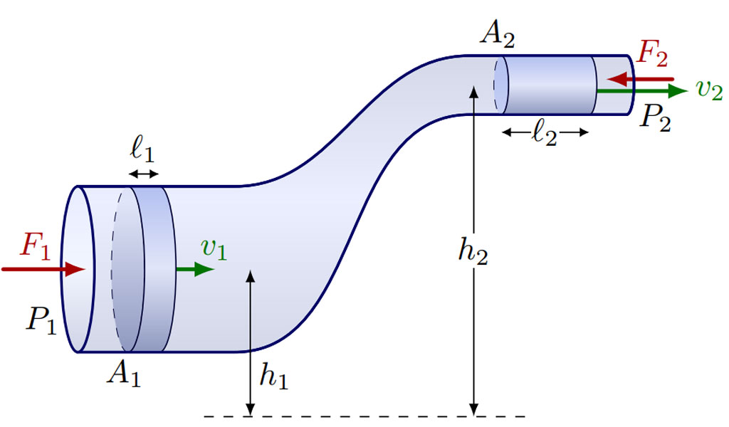
Bernoulli’s equation can be derived by applying the principle of conservation of energy to a fluid flow along a streamline. A streamline is an imaginary line that represents the path traced by a fluid particle as it moves through the flow field without crossing any other streamlines. The derivation is based on the following assumptions:
Assumptions and Limitations
- Incompressible and Inviscid Fluid: The derivation assumes that the fluid is incompressible, meaning its density remains constant, and inviscid, implying there is no internal friction or viscosity within the fluid.
- Steady State Flow: The fluid flow is assumed to be steady, meaning the fluid properties at any given point in the flow field do not change with time.
- Along a Streamline: The derivation is applicable only along a single streamline, where the fluid particles move in the same direction and experience the same conditions.
- No External Forces: The fluid flow is assumed to be free of external forces other than gravity, so that work done by forces other than pressure forces is negligible.
The Conservation of Energy Principle
The derivation of Bernoulli’s equation is based on the principle of conservation of energy applied to a fluid particle along a streamline. The total energy of the fluid particle remains constant as it moves through the flow field. The total energy of the fluid particle consists of three components:
- Pressure Energy: This component represents the pressure of the fluid at the particular point on the streamline. It is the energy associated with the fluid particle’s position in the flow field relative to a reference pressure.
- Kinetic Energy: This component represents the energy associated with the fluid particle’s motion. It is proportional to the square of the fluid velocity at that point on the streamline.
- Potential Energy: This component represents the energy due to the fluid particle’s elevation above a reference level. It is proportional to the fluid particle’s height above the reference level and its weight due to gravity.
Interpretation of Terms in the Equation
- Pressure Term (P): The pressure term represents the static pressure of the fluid at a particular point on the streamline. It is the force per unit area exerted by the fluid on its surroundings. An increase in pressure corresponds to a decrease in fluid velocity, and vice versa.
- Kinetic Energy Term (\frac{1}{2}\rho v^221ρv2): The kinetic energy term represents the energy associated with the motion of the fluid particle. It is proportional to the square of the fluid velocity and indicates that an increase in fluid velocity leads to an increase in kinetic energy.
- Potential Energy Term (\rho ghρgh): The potential energy term represents the energy due to the fluid particle’s position above a reference level. It takes into account the fluid particle’s elevation and its weight due to gravity. An increase in elevation leads to an increase in potential energy.
The Bernoulli’s equation allows us to understand the interplay between pressure, velocity, and elevation in a moving fluid. It is a fundamental concept in fluid dynamics and has wide-ranging applications in various fields, including aviation, hydraulics, weather prediction, and medical sciences. However, it is important to remember that the equation’s derivation is based on idealized assumptions, and its application is limited to certain scenarios where these assumptions hold true.
Real-World Applications of Bernoulli’s Equation
Bernoulli’s equation is a fundamental principle in fluid dynamics that finds numerous real-world applications in various fields. Let’s explore some of the key applications of Bernoulli’s equation in different domains:
Aviation and Aerodynamics
- Lift and the Bernoulli Effect: One of the most significant applications of Bernoulli’s equation in aviation is explaining lift generation on airplane wings. As an aircraft moves through the air, the shape of its wings causes the airflow to be faster over the upper surface compared to the lower surface. According to Bernoulli’s equation, this difference in airflow velocity results in a difference in pressure between the upper and lower surfaces of the wing. The lower pressure on the upper surface creates an upward lift force that helps keep the aircraft airborne.
- Aircraft Design and Performance: Engineers and aircraft designers use Bernoulli’s equation to optimize wing design, airfoil profiles, and control surfaces to maximize lift and improve aircraft performance. Understanding the relationship between pressure, velocity, and lift is essential in designing efficient and safe airplanes.
Hydraulics and Fluid Machinery
- Hydraulic Principles and Systems: Bernoulli’s equation is fundamental in designing and analyzing hydraulic systems. It helps in understanding pressure changes, flow rates, and energy losses in pipes, channels, and hydraulic components.
- Water Turbines and Pumps: Water turbines, such as hydroelectric turbines, and pumps rely on Bernoulli’s equation to optimize their efficiency and output. The equation is used to determine the pressure and velocity changes across the turbine or pump blades, aiding in their design and performance analysis.
Weather Phenomena
- The Formation of Clouds and Wind Patterns: Bernoulli’s equation plays a role in understanding the formation of clouds and wind patterns. For example, as air rises in the atmosphere, it expands due to reduced pressure at higher elevations, leading to adiabatic cooling. This process is crucial in cloud formation and precipitation.
- Cyclones and Anticyclones: In meteorology, Bernoulli’s equation is used to explain the dynamics of cyclones and anticyclones. Airflow patterns around these weather systems are influenced by pressure gradients, which can be analyzed using Bernoulli’s equation.
Medical and Biological Applications:
- Blood Flow and Cardiovascular Systems: Bernoulli’s equation is applied in medicine to understand blood flow through arteries and veins. It helps in assessing blood pressure, flow velocity, and potential obstructions or irregularities in blood vessels.
- Respiratory System and Breathing Mechanism: The principles of Bernoulli’s equation are used to explain the mechanics of breathing. As air flows through the airways and over the vocal cords, variations in pressure and airflow velocity are critical for speech production and respiration.
Bernoulli’s equation is a versatile and powerful tool that finds a wide range of real-world applications in aviation, hydraulics, meteorology, and medical sciences. Its ability to explain fluid behavior and the interplay between pressure, velocity, and elevation makes it indispensable for engineers, scientists, and researchers in various fields. By understanding and applying Bernoulli’s equation, we can design more efficient aircraft, optimize hydraulic systems, predict weather patterns, and gain valuable insights into the dynamics of biological systems.
Experimental Verification of Bernoulli’s Equation
Experimental verification of Bernoulli’s equation is crucial to validate its applicability in real-world scenarios and to understand the complex behavior of fluid flow. Several experimental methods have been developed to demonstrate the principles of Bernoulli’s equation and to investigate various fluid flow phenomena. Let’s explore some of the key experimental techniques used for verifying Bernoulli’s equation and the challenges and limitations associated with these experiments:
Venturi Effect and Pitot Tubes:
- Venturi Effect: The Venturi effect is a classic example of Bernoulli’s equation in action. It demonstrates how the fluid’s velocity increases and its pressure decreases as it flows through a constriction (narrowing) in a pipe. To experimentally verify this effect, a Venturi tube is used, which consists of a gradually narrowing section in the middle of a pipe. By measuring the pressure difference between the wider and narrower sections, one can confirm the principles of Bernoulli’s equation.
- Pitot Tubes: Pitot tubes are devices used to measure the velocity of a fluid flow. They work based on Bernoulli’s equation by comparing the total pressure (static pressure plus dynamic pressure) of the fluid at a stagnation point (where the flow velocity is zero) with the static pressure at another point in the flow. This difference in pressure allows for the determination of the flow velocity.
Wind Tunnels and Fluid Flow Visualization
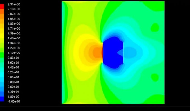
- Wind Tunnels: Wind tunnels are essential tools for experimental fluid dynamics. They are used to simulate and study airflow around objects, such as aircraft wings and cars, at various velocities and angles of attack. Wind tunnels help researchers validate Bernoulli’s equation by measuring pressure distributions and velocity profiles around the model under study.
- Fluid Flow Visualization: Visualization techniques, such as using dye injection or smoke particles, allow researchers to visualize and understand complex fluid flow patterns. By observing how fluids behave around obstacles or through various geometries, researchers can gain insights into the principles of Bernoulli’s equation and validate its predictions.
Challenges and Limitations in Experimental Validation
- Viscosity and Compressibility: Bernoulli’s equation assumes that the fluid is inviscid (no internal friction) and incompressible (constant density). However, real fluids have viscosity, which can affect the flow behavior and introduce deviations from ideal conditions. Additionally, for high-speed flows, the assumption of incompressibility may not hold, requiring modifications to the equation.
- Turbulence and Boundary Layer Effects: Fluid flows in practical situations are often turbulent, especially around complex geometries. Turbulence can significantly affect pressure distributions and flow patterns, leading to challenges in obtaining accurate experimental results that precisely match the predictions of Bernoulli’s equation. Similarly, the boundary layer, which forms near solid surfaces, can impact flow characteristics and require special consideration.
- Energy Losses and Friction: Real-world fluid systems inevitably experience energy losses due to friction and other factors. These losses are not accounted for in the idealized Bernoulli’s equation. Therefore, experimental verification should consider energy losses and compare them to theoretical predictions.
- Mach Number Effects: For fluid flows with high velocities, the Mach number (the ratio of flow velocity to the speed of sound) becomes significant. In such cases, compressibility effects need to be considered, and alternative equations, such as the Euler equations or the Navier-Stokes equations, may be used instead of the simplified Bernoulli’s equation.
Despite these challenges and limitations, experimental verification of Bernoulli’s equation remains essential for refining our understanding of fluid behavior and its practical applications. By combining experimental data with theoretical analysis and computational simulations, researchers can gain a more comprehensive understanding of fluid dynamics and its underlying principles.
Extension and Modification of Bernoulli’s Equation
Extension and modification of Bernoulli’s equation is necessary to address specific scenarios involving compressible fluids, viscous fluids, and two-phase fluid systems. The idealized Bernoulli’s equation, derived under the assumptions of incompressible and inviscid fluid flow, may not be applicable in these situations. Let’s explore the extensions and modifications of Bernoulli’s equation for these cases:
Compressible Fluid Flows:
In cases where the fluid velocity approaches or exceeds the speed of sound, compressibility effects become significant, and the idealized Bernoulli’s equation is no longer valid. For compressible fluid flows, the appropriate equation is derived from the Euler equations or the Navier-Stokes equations, which account for changes in fluid density due to pressure and velocity variations. The modified equation is known as the compressible Bernoulli’s equation and is written as:
P+21ρv2+ρgh=constant
Where: PP = Pressure of the fluid
\rhoρ = Density of the fluid
vv = Velocity of the fluid
gg = Acceleration due to gravity
hh = Elevation or height of the fluid
In compressible fluid flows, changes in pressure can lead to substantial variations in fluid density, which must be considered in the equation.
Viscous Fluid Flows and Reynolds Number:
When dealing with viscous fluid flows, where internal friction (viscosity) plays a significant role, the idealized Bernoulli’s equation is inadequate. Viscous effects can cause energy losses due to shear forces and boundary layer interactions. The modified Bernoulli’s equation for viscous flows is derived from the Navier-Stokes equations, taking into account the viscous stresses. It is written as:
P+21ρv2+ρgh+ρτ=constant
Where: \tauτ = Shear stress due to viscosity
The viscous term (\frac{\tau}{\rho}ρτ) accounts for the energy losses due to viscosity, and its inclusion in the equation is essential for accurate predictions in viscous fluid flows.
The Reynolds number (Re) is a dimensionless parameter that characterizes the flow regime, whether it is laminar or turbulent. In situations where Re is high (turbulent flow), the viscous term becomes relatively small compared to the other terms, and the equation simplifies to the idealized Bernoulli’s equation. However, for low Re (laminar flow), the viscous term becomes significant and can significantly affect the flow behavior.
Application in Two-phase Fluid Systems:
In two-phase fluid systems, such as gas-liquid flows or liquid-liquid flows, the idealized Bernoulli’s equation needs modification to consider the interactions and energy exchanges between the two phases. The modification involves incorporating additional terms that account for the specific characteristics of each phase and their interactions.
For gas-liquid flows, the equation may include terms for interfacial forces and phase change effects. In liquid-liquid flows, additional terms may account for density differences and interactions at the phase interface.
Due to the complexities of two-phase flows, including the possibility of phase separation, cavitation, and bubble dynamics, more sophisticated models and numerical simulations are often required to accurately predict the behavior of such systems.
While the idealized Bernoulli’s equation is a powerful tool for understanding fluid behavior in incompressible and inviscid flows, its application is limited to these specific conditions. For compressible, viscous, and two-phase fluid flows, extensions and modifications of the equation are necessary to account for additional factors and ensure accurate predictions. These modified equations, derived from more comprehensive fluid dynamics equations, play a vital role in solving real-world engineering and scientific problems involving complex fluid systems.
Numerical Methods in Solving Bernoulli’s Equation
Numerical methods play a crucial role in solving fluid dynamics problems, including Bernoulli’s equation, especially when analytical solutions are not feasible or practical. Two common numerical techniques used for solving fluid flow equations, including Bernoulli’s equation, are Finite Difference Methods and Computational Fluid Dynamics (CFD).
Finite Difference Methods:
Finite Difference Methods (FDM) are a class of numerical techniques used to approximate the derivatives of a function. In the context of fluid dynamics, FDM is employed to discretize the differential equations governing fluid flow, including Bernoulli’s equation, into algebraic equations. These algebraic equations are then solved iteratively to obtain numerical solutions.
To apply FDM to Bernoulli’s equation, the spatial domain is discretized into a grid, and the partial derivatives with respect to space are replaced by finite difference approximations. The time derivatives, if applicable (for unsteady flows), can also be handled using time-stepping schemes.
For example, consider the 1D steady-state form of Bernoulli’s equation in a pipe:
P+21ρv2+ρgh=constant
The spatial derivative (\frac{\partial v}{\partial x}∂x∂v) can be approximated using a finite difference scheme, such as central difference or upwind difference. The algebraic equations obtained after discretization can be solved using iterative methods like the Gauss-Seidel method or the Successive Over-Relaxation (SOR) method.
Finite Difference Methods are relatively straightforward to implement and computationally efficient for simple geometries and flow problems. However, they may face challenges when dealing with complex geometries and unstructured grids, where other numerical methods like Computational Fluid Dynamics (CFD) become more suitable.
Computational Fluid Dynamics (CFD):
CFD is a more advanced numerical technique used to solve fluid flow problems, including Bernoulli’s equation, in complex geometries and under various flow conditions. CFD involves discretizing the fluid domain into a mesh (structured or unstructured) and numerically solving the Navier-Stokes equations or the Euler equations, which are the fundamental governing equations of fluid dynamics.
In CFD, the partial derivatives in the Navier-Stokes equations are approximated using finite difference, finite volume, or finite element methods. The resulting system of algebraic equations is solved using iterative or direct numerical methods.
CFD simulations can handle both steady-state and time-dependent (unsteady) flows, turbulence, compressibility, and complex boundary conditions. With advances in computing power, CFD has become an indispensable tool in engineering design, aerodynamics, hydrodynamics, and other fields involving fluid flow analysis.
CFD software packages provide user-friendly interfaces, enabling engineers and researchers to set up and simulate fluid flow problems without delving into the intricacies of numerical methods. These tools also offer visualization and post-processing capabilities to interpret and analyze the results effectively.
Numerical methods, such as Finite Difference Methods and Computational Fluid Dynamics (CFD), have revolutionized fluid dynamics by enabling the simulation and analysis of complex fluid flow problems. These methods provide valuable insights into fluid behavior, especially in situations where analytical solutions are unavailable or impractical. Engineers and scientists rely on these numerical techniques to optimize designs, understand flow phenomena, and predict fluid behavior in a wide range of real-world applications.
Challenges and Limitations of Bernoulli’s Equation
While Bernoulli’s equation is a powerful tool for understanding fluid behavior in certain situations, it has several challenges and limitations that restrict its applicability to certain fluid flow scenarios. Some of the key challenges and limitations of Bernoulli’s equation are as follows:
Turbulent Flow and Instabilities
Bernoulli’s equation assumes laminar flow, where fluid particles move in parallel layers in a smooth, orderly manner. However, in real-world scenarios, fluid flows can often be turbulent, characterized by chaotic and irregular fluctuations in velocity and pressure. Turbulence leads to significant energy losses and complicates the application of Bernoulli’s equation. The presence of vortices, eddies, and turbulent mixing invalidates the simplified assumptions underlying Bernoulli’s equation.
Non-Ideal Fluids and Phase Changes
Bernoulli’s equation is derived based on the assumptions of incompressible and inviscid fluid flow. In reality, many fluids are compressible, and viscosity (internal friction) plays a significant role. For example, in gases or fluids undergoing phase changes (e.g., vaporization, condensation), the idealized assumptions may not hold. Additionally, fluids with non-constant density, like compressible gases, cannot be accurately analyzed using the standard Bernoulli’s equation.
High-Speed Flows and Shock Waves
At high flow velocities, especially when the fluid approaches or exceeds the speed of sound, compressibility effects become significant, and shock waves may form. Shock waves are abrupt pressure and velocity changes that cannot be accurately predicted using Bernoulli’s equation. For high-speed flows, more advanced equations, such as the compressible Euler or Navier-Stokes equations, are required.
Energy Losses and Friction
Bernoulli’s equation assumes an idealized, frictionless flow with no energy losses. In reality, energy is dissipated due to friction between the fluid and the boundaries of the flow path. The presence of energy losses due to viscous forces, heat transfer, and other factors must be considered for accurate predictions, especially in practical engineering applications.
Steady-State and Incompressible Flow
Bernoulli’s equation is valid for steady-state flow, where fluid properties at a given point do not change with time. It is also applicable to incompressible flows, where the fluid density remains constant. However, many real-world scenarios involve unsteady flows and compressible fluids, necessitating the use of more complex equations, such as the time-dependent Navier-Stokes equations.
While Bernoulli’s equation is a valuable and widely used tool in fluid dynamics, it is essential to be aware of its limitations and applicability. Engineers and scientists must exercise caution when using Bernoulli’s equation in practical scenarios that involve turbulence, non-ideal fluids, high-speed flows, and shock waves. For more complex situations, such as those encountered in aerodynamics, gas dynamics, and supersonic flows, advanced equations, numerical methods, and computational fluid dynamics (CFD) simulations are more appropriate for accurate predictions and analysis.
The Enduring Impact of Bernoulli’s Equation:
Bernoulli’s equation has left an indelible mark on the study of fluid dynamics and its applications. Its simplicity and elegance make it a valuable tool for engineers, scientists, and researchers across diverse fields. From aircraft design to medical diagnostics, Bernoulli’s equation continues to play a crucial role in understanding and predicting fluid behavior.
The equation’s enduring impact lies in its ability to provide valuable insights into fluid flow patterns, pressure distributions, and energy considerations. It has paved the way for advancements in aerodynamics, hydraulics, meteorology, and medical sciences, among others. The principles of Bernoulli’s equation are taught at various educational levels, shaping the understanding of fluid mechanics for generations of students and professionals.
As technology and computational capabilities continue to advance, researchers are exploring more complex and sophisticated numerical methods for fluid flow analysis. Numerical simulations using CFD are becoming increasingly prevalent for understanding fluid behavior in intricate geometries and unsteady flows. With the advent of high-performance computing, simulations can provide detailed visualizations and data that were once unimaginable.
Research frontiers in fluid dynamics involve exploring turbulence modeling, multiphase flows, and the interplay of fluid dynamics with other scientific domains, such as biology and climate science. Understanding and mitigating turbulence, which remains one of the most challenging aspects of fluid dynamics, have substantial implications in engineering design and energy efficiency.
Moreover, the integration of fluid dynamics with emerging technologies like artificial intelligence and machine learning presents exciting opportunities. These technologies can enhance the accuracy and efficiency of fluid flow simulations and enable faster optimization of engineering designs.
The legacy of Bernoulli’s equation continues to shape the study of fluid dynamics and inspire new discoveries. As researchers delve into more complex fluid flow scenarios and embrace cutting-edge computational methods, the potential for breakthroughs in fluid dynamics research remains boundless.