
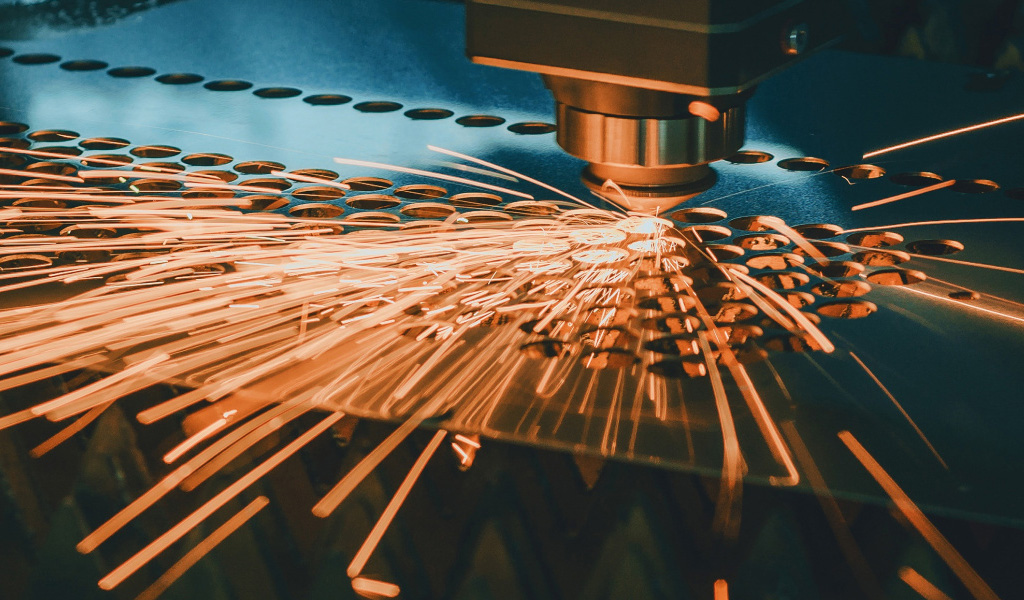
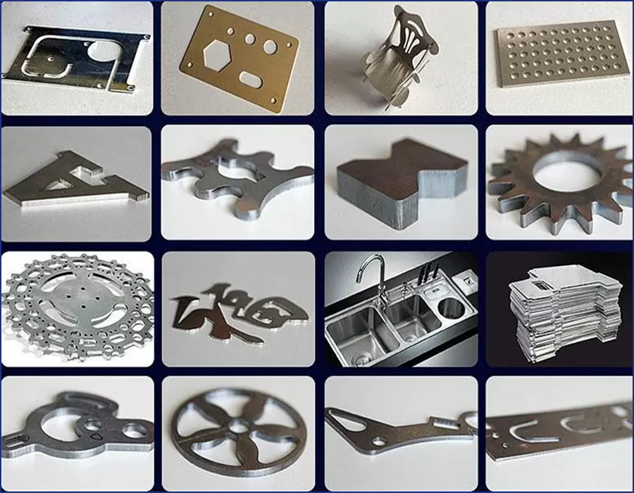
Laser cutting is a widely utilized thermal processing technique in modern manufacturing, prized for its precision, efficiency, and versatility across a range of materials, including metals, polymers, and composites.
Central to the laser cutting process is the interaction between a focused laser beam and the workpiece, where energy is absorbed, leading to melting, vaporization, or sublimation of the material. However, not all energy delivered by the laser contributes to material removal; a significant portion is lost through heat conduction into the surrounding workpiece, influencing the cut quality, heat-affected zone (HAZ), and overall process efficiency.
Understanding and quantifying this heat conduction loss is critical for optimizing laser cutting parameters and developing predictive models. The numerical calculation method provides a robust framework for estimating these losses by solving the governing heat transfer equations under complex boundary conditions. This article explores the theoretical basis, mathematical formulations, numerical techniques, and practical implementations of such methods, with detailed comparisons to enhance scientific understanding.
Fundamentals of Heat Conduction in Laser Cutting
Heat conduction in laser cutting arises from the thermal energy imparted by the laser beam, which is typically modeled as a moving heat source with a Gaussian or uniform intensity distribution. As the beam traverses the workpiece, energy is absorbed at the surface, raising the local temperature to levels sufficient for material removal. However, the high thermal gradients established near the cutting front drive heat diffusion into the adjacent material, a process governed by the heat conduction equation. This equation, derived from Fourier’s law of heat conduction, describes the spatial and temporal evolution of temperature within a medium:
ρcp{∂t/∂T}=∇⋅(k∇T)+Q
where:
ρ is the material density (kg/m³),
cp is the specific heat capacity (J/kg·K),
T is the temperature (K),
t is time (s),
k is the thermal conductivity (W/m·K),
Q is the volumetric heat source term (W/m³),
∇ denotes the spatial gradient operator.
In laser cutting, Q Q Q represents the laser energy absorbed by the material, often approximated as a surface flux adjusted for absorption efficiency. The heat conduction loss is the portion of this energy that diffuses away from the cutting zone rather than contributing to material removal, quantified as the conductive heat flux into the workpiece.
The complexity of laser cutting stems from its three-dimensional, transient nature, coupled with material phase changes (melting or vaporization) and the moving boundary of the cut front. Analytical solutions to the heat conduction equation are feasible only under simplified assumptions—such as a semi-infinite medium or steady-state conditions—limiting their applicability to real-world scenarios. Numerical methods, by contrast, offer the flexibility to handle these complexities, making them indispensable for accurate estimation of heat conduction losses.
Theoretical Framework for Heat Conduction Loss
To calculate heat conduction loss numerically, the problem must be framed within a coordinate system that reflects the geometry of the cutting process. Typically, a Cartesian coordinate system is employed, with the laser beam moving along the x x x-axis, the y y y-axis perpendicular to the cutting direction in the plane of the workpiece, and the z z z-axis aligned with the beam direction through the material thickness. The heat conduction equation in Cartesian coordinates becomes:
ρcp{∂t/∂T}={∂/x∂}{k(∂x∂T)}+∂/∂y{k(∂y∂T)}+∂/∂z{k(∂z∂T}+Q(x,y,z,t)
The heat source Q Q Q is often modeled as a Gaussian distribution for continuous-wave lasers:
Q(x,y,z,t)={2ηP/[πr(2/b)]}e−rb22(x−vt)2+y2δ(z)
where:
η is the absorption coefficient,
P is the laser power (W),
rb is the beam radius (m),
v is the cutting speed (m/s),
δ(z) is the Dirac delta function, localizing the heat input at the surface (z
z = 0 z=0).
Heat conduction loss is determined by integrating the conductive heat flux over the boundaries of the cutting zone, typically the kerf walls and the subsurface region. The flux is given by Fourier’s law:
q=−k∇T
The total conduction loss Qcond (W) is then:
Qcond=∫A−k∇T⋅ndA
where A A A is the surface area surrounding the cutting zone, and n \mathbf{n} n is the outward normal vector. Numerically, this integral is evaluated over a discretized domain, requiring careful definition of boundary conditions and material properties.
Boundary and Initial Conditions
Accurate numerical modeling necessitates appropriate boundary and initial conditions. The top surface (z=0 z = 0 z=0) experiences the laser heat flux, modified by convective and radiative losses:
−k(∂z/∂T)/z=0=ηqlaser−h(T−T∞)−ϵσ(T4−T∞4)
where:
- qlaser q_{\text{laser}} qlaser is the incident laser flux (W/m²),
- h h h is the convective heat transfer coefficient (W/m²·K),
- T∞ T_\infty T∞ is the ambient temperature (K),
- ϵ \epsilon ϵ is the emissivity,
- σ \sigma σ is the Stefan-Boltzmann constant (5.67 × 10⁻⁸ W/m²·K⁴).
At the kerf walls, where material is removed, a Neumann boundary condition may apply, assuming negligible heat loss through the cut, or a temperature condition if melting is modeled explicitly (e.g., T=Tm T = T_m T=Tm, the melting temperature). The bottom surface (z=d z = d z=d, where d d d is the workpiece thickness) and lateral boundaries are often treated as convective or insulated, depending on the setup. The initial condition is typically a uniform ambient temperature:
T(x,y,z,0)=T∞
Numerical Methods for Solving the Heat Conduction Equation
Several numerical techniques are employed to solve the heat conduction equation in laser cutting, each with distinct advantages and trade-offs. The most common methods include the Finite Difference Method (FDM), Finite Element Method (FEM), and Finite Volume Method (FVM), with adaptations to handle the moving heat source and phase changes.
Finite Difference Method (FDM)
The FDM discretizes the spatial and temporal domains into a grid, approximating derivatives with difference equations. For a 2D simplification (assuming symmetry or thin sheets), the explicit FDM scheme for the heat equation is:
Ti,jn+1=Tn/i,j+(Δx)2αΔt(Ti+1,jn−2Ti,jn+Ti−1,jn)+(Δy)2αΔt(Ti,j+1n−2Ti,jn+Ti,j−1n)+ρcpΔtQi,jn
where:
- Ti,jn T_{i,j}^n Ti,jn is the temperature at grid point (i,j) (i, j) (i,j) and time step n n n,
- α=k/(ρcp) \alpha = k / (\rho c_p) α=k/(ρcp) is the thermal diffusivity (m²/s),
- Δt \Delta t Δt, Δx \Delta x Δx, and Δy \Delta y Δy are the time and spatial step sizes.
The explicit scheme is straightforward but conditionally stable, requiring Δt (the Courant-Friedrichs-Lewy condition). Implicit schemes, such as the Crank-Nicolson method, offer unconditional stability but require solving a system of linear equations at each step, increasing computational cost.
Finite Element Method (FEM)
The FEM divides the domain into elements (e.g., triangles or tetrahedra), approximating the temperature field with basis functions. The weak form of the heat equation is solved using Galerkin’s method, yielding a system of equations:
[M]{T˙}+[K]{T}={F} [M] \{\dot{T}\} + [K] \{T\} = \{F\} [M]{T˙}+[K]{T}={F}
where:
- [M] [M] [M] is the mass matrix,
- [K] [K] [K] is the stiffness matrix (incorporating conductivity),
- {F} \{F\} {F} is the force vector (including the heat source),
- {T} \{T\} {T} and {T˙} \{\dot{T}\} {T˙} are the temperature and its time derivative.
FEM excels in handling irregular geometries and adaptive meshing near the cutting front, though it is computationally intensive. Commercial software like ANSYS or COMSOL often implements FEM for laser cutting simulations.
Finite Volume Method (FVM)
The FVM conserves energy over control volumes, integrating the heat equation over each cell:
ρcp∂∂t∫VT dV=−∫∂Vk∇T⋅n dA+∫VQ dV \rho c_p \frac{\partial}{\partial t} \int_V T \, dV = -\int_{\partial V} k \nabla T \cdot \mathbf{n} \, dA + \int_V Q \, dV ρcp∂t∂∫VTdV=−∫∂Vk∇T⋅ndA+∫VQdV
Discretization yields a balance equation for each cell, solved iteratively. FVM is particularly suited for heat transfer problems due to its conservation properties and is widely used in computational fluid dynamics (CFD) codes adapted for thermal analysis.
Incorporating the Moving Heat Source
The laser’s motion introduces a dynamic heat source, often handled by shifting the source term Q Q Q with velocity v v v in the numerical grid. Alternatively, a coordinate transformation to a moving reference frame simplifies the problem:
x′=x−vt,y′=y,z′=z x’ = x – v t, \quad y’ = y, \quad z’ = z x′=x−vt,y′=y,z′=z
The heat equation adjusts to:
ρcp(∂T∂t−v∂T∂x′)=∇⋅(k∇T)+Q(x′,y′,z′,t) \rho c_p \left( \frac{\partial T}{\partial t} – v \frac{\partial T}{\partial x’} \right) = \nabla \cdot (k \nabla T) + Q(x’, y’, z’, t) ρcp(∂t∂T−v∂x′∂T)=∇⋅(k∇T)+Q(x′,y′,z′,t)
This approach reduces numerical complexity but requires careful boundary condition adjustments.
Dimensionless Analysis and the Peclet Number
To generalize results, dimensionless parameters are introduced, notably the Peclet number (Pe Pe Pe), which compares convective to diffusive heat transport:
ρcp∂t∂∫VTdV=−∫∂Vk∇T⋅ndA+∫VQdV
where L L L is a characteristic length (e.g., beam radius or material thickness). In laser cutting, Pe Pe Pe is interpreted as a dimensionless cutting speed. Studies suggest that conduction loss correlates strongly with Pe Pe Pe, with empirical correlations like:
QcondP=0.5+0.868Pe(0.2≤Pe≤10) \frac{Q_{\text{cond}}}{P} = 0.5 + \frac{0.868}{Pe} \quad (0.2 \leq Pe \leq 10) PQcond=0.5+Pe0.868(0.2≤Pe≤10)
This relation, derived from integral methods, highlights that slower cutting speeds (lower Pe Pe Pe) increase conduction losses relative to laser power.
Practical Implementation and Validation
Implementing these numerical methods involves discretizing the domain, selecting a time-stepping scheme, and iterating until convergence. For a steel plate (e.g., k=50 W/m\cdotpK k = 50 \, \text{W/m·K} k=50W/m\cdotpK, ρ=7850 kg/m³ \rho = 7850 \, \text{kg/m³} ρ=7850kg/m³, cp=500 J/kg\cdotpK c_p = 500 \, \text{J/kg·K} cp=500J/kg\cdotpK), with a 1 kW laser (rb=0.1 mm r_b = 0.1 \, \text{mm} rb=0.1mm, v=0.01 m/s v = 0.01 \, \text{m/s} v=0.01m/s), with a 1 kW laser (rb=0.1 mm r_b = 0.1 \, \text{mm} rb=0.1mm, v=0.01 m/s v = 0.01 \, \text{m/s} v=0.01m/s), a 3D FVM model might use a grid of 100 × 100 × 50 cells, with Δt=10−5 s \Delta t = 10^{-5} \, \text{s} Δt=10−5s. The resulting temperature field reveals a HAZ extending 0.5–1 mm, with conduction losses of 20–30% of input power, validated against thermocouple measurements.
Comparative Analysis of Numerical Methods
The choice of numerical method impacts accuracy, computational cost, and applicability. Below is a detailed comparison:
| Method | Accuracy | Computational Cost | Ease of Implementation | Best Suited For |
|---|---|---|---|---|
| FDM (Explicit) | Moderate (grid-dependent) | Low | High | Simple geometries, rapid prototyping |
| FDM (Implicit) | High (stable) | Moderate | Moderate | Steady-state problems |
| FEM | Very High (adaptive) | High | Low (requires software) | Complex geometries, phase changes |
| FVM | High (conservative) | Moderate to High | Moderate | Thermal-fluid coupling, industrial use |
| Parameter | FDM (Explicit) | FDM (Implicit) | FEM | FVM |
|---|---|---|---|---|
| Grid Size | 100 × 100 × 50 | 100 × 100 × 50 | 10⁵ elements | 10⁵ cells |
| Time Step (s) | 10⁻⁵ | 10⁻⁴ | 10⁻⁴ | 10⁻⁴ |
| Runtime (min) | 5 | 15 | 60 | 30 |
| HAZ Error (%) | 10–15 | 5–10 | 2–5 | 5–8 |
| Loss Estimate (%) | 25–35 | 20–30 | 18–25 | 20–28 |
These tables illustrate FEM’s superior accuracy at the expense of computational resources, while FDM offers a quick, albeit less precise, alternative. FVM balances both, making it prevalent in industrial applications.
Future Directions
Numerical calculation of heat conduction loss informs parameter optimization—e.g., increasing v v v to reduce Pe Pe Pe and thus Qcond Q_{\text{cond}} Qcond—and predicts HAZ size, critical for quality control in aerospace or automotive manufacturing. However, limitations include assumptions of constant material properties (neglecting temperature dependence), simplified boundary conditions, and computational demands for real-time control. Advanced models incorporating phase change enthalpies or adaptive grids mitigate some issues but increase complexity.
Emerging techniques, such as machine learning integration with numerical solvers, promise faster predictions by training on simulation data. Hybrid methods combining FVM with analytical solutions for specific regions (e.g., far-field conduction) could further enhance efficiency. As laser technology advances, with higher powers and dynamic beam shaping, numerical models must evolve to capture these effects accurately.
The Detail Of BE-CU Laser Cutting Company
BE-CU.COM Laser Cutting provides services to a wide network of industries and markets. BE-CU is uniquely positioned to Laser Cut, Laser Engrave, Precision CNC Machine and Precision Finish Grind parts and components.We use large format industrial laser cutting machines that are extremely precise with up to .001” tolerance. Not only we cut and engrave your project, we are ready to answer any questions you may have about the process and give you expert advice.
So, reach out even if you’re unsure of your specific need or if you think you may require a different type of manufacturing service(as laser cutting medical parts). Laser cutting service by BE-CU makes ordering your parts simple. Just upload your CAD files onto the platform for an instant price and lead time. Our mission is to save engineers’ time for value-adding activities.
-
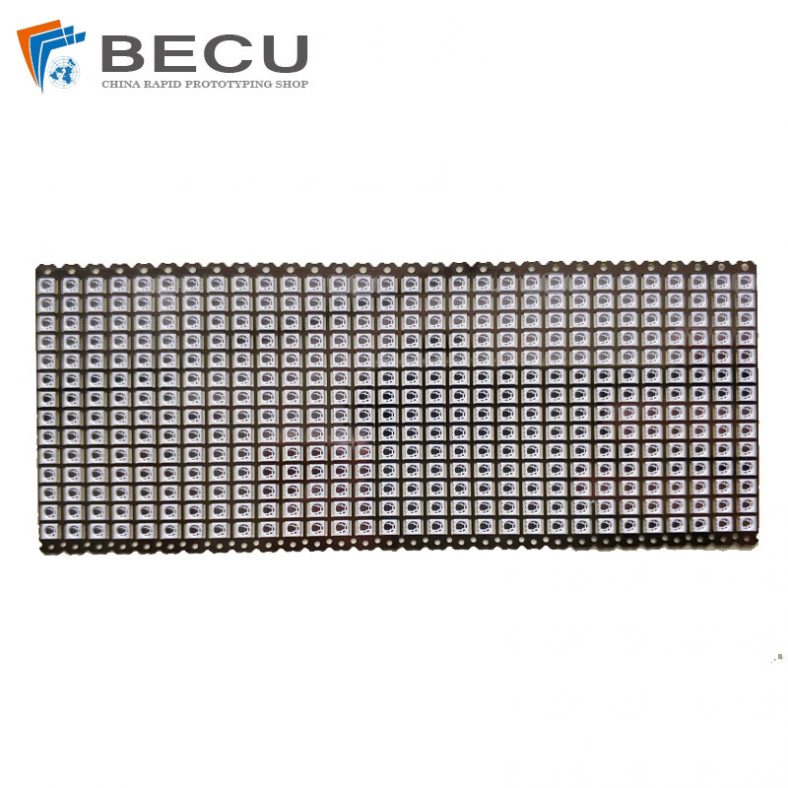
Etching LED EMC Packaging Bracket
-
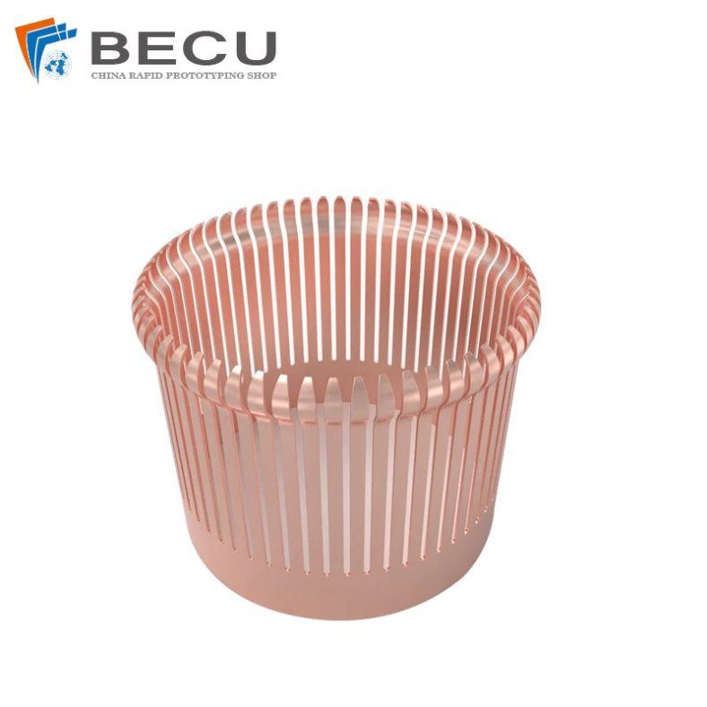
Etching Low Resistivity Copper 110 Contact Rings
-
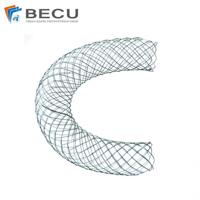
Laser Cut Nitinol Stent For Bile Duct
-
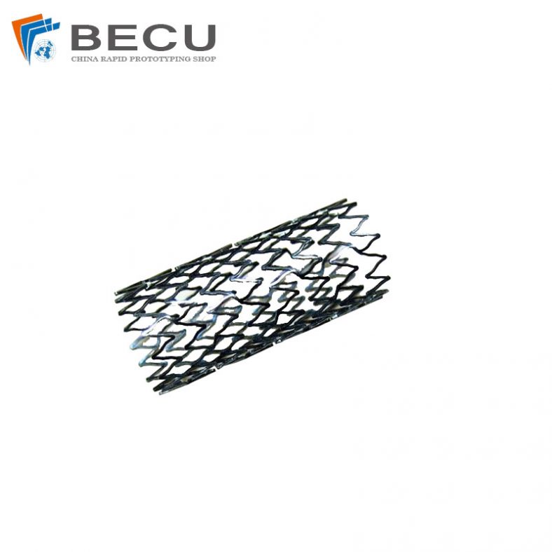
Stents For Carrying Valves And Venous Valve Replacement Devices
-
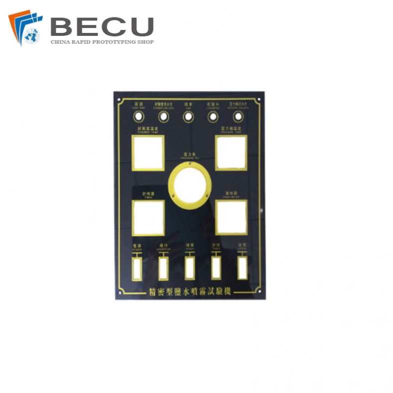
Laser Cutting PC Anti-Static Membrane Switch
-
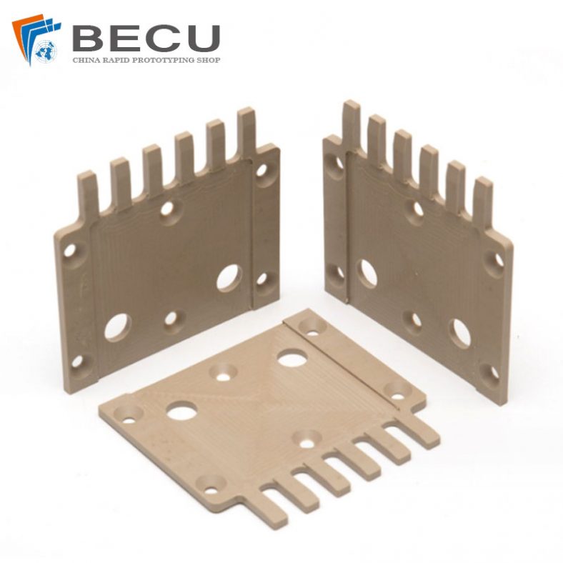
Precision Engraving Special-Shaped Natural Color PEEK Parts
-
Acrylic Laser Cut Signs
-

Acrylic Laser Cut Earrings